⏳ Mining deep into Data Mining - Statistics - PART II ⏳
Before analyzing distributions in statistics, Let's understand the required essential basics
💭 MEAN
Mean is an essential concept in statistics. In common terms, it can be defined as the average of a collection of values. It can be referred to as central tendency or centrality for a probability distribution. Thus, it basically denotes the centrality of a series of values.
💭 STANDARD DEVIATION
A standard deviation is a statistic that measures the dispersion of a dataset relative to its mean. The standard deviation is calculated as the square root of variance by determining each data point's deviation relative to the mean.
💭 VARIANCE
Variance is the measure of how well the data is dispersed from the existing data points. (ie) the mean squared difference between every data point and the center of distribution (mean). This yields the rate of dispersion of data points. Variance is also the square of standard deviation.
For example, let's consider a series of price list values of multiple products in a supermarket.
price_list = [87.56, 56.78, 98.76, 56.43, 32.12, 76, 90, 43.45, 76.23, 12.05]
Mean = sum of price_list / number of entries in price_list
MEAN = SUM(price_list) / LEN(price_list)
Variance = for each value v in the list, perform square of the difference between the element and the mean (ie) square of (v - mean), finally perform a summation
VARIANCE = SUM(square of (v - mean) for every v in price_list) / LEN(price_list)
Standard deviation = Perform the square root of the variance
STD = SQRT(variance)

Let us assume, the height of 5 dogs are calculated. (Reference & Image Source: Internet)
👉 The GREEN line represents the mean or average height of the dogs.
👉 The difference between the INVERTED RED indicator and the mean denotes the variance.
👉 The square root of the variance (would be less than the variance) - the BLUE line is the threshold value, thus the standard deviation would be the square root of the sum of the difference of every value against the total values (ie) the square root of variance.
Let's understand what distribution is all about 💪
DISTRIBUTION
A distribution in statistics is a function that shows the possible values for a variable and how often they occur. Let's assume a die numbered from 1 to 6. When rolling the die, there are possibilities that values from 1 to 6 might appear on the dice. Thus, the distribution of an event consists not only of the input values that can be observed but is made up of all possible values.
Based on the type of data being dealt with, there are two different types of distribution - Discrete and Continuous distribution.
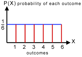
👉 DISCRETE UNIFORM DISTRIBUTION - Outcomes are likely to be equal
In simple terms, uniform distribution refers to cases where the outcomes are likely to be equal. Let us consider the scenario of rolling a die, there is an equal possibility of the values 1, 2, 3, 4, 5, and 6 appearing in the next throw. Thus, the probability is 1/6 or 0.16666.
The figure below shows the equal likeliness of the outcomes (Image Source: Internet)
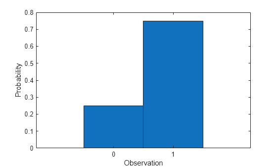
👉 BERNOULLI DISTRIBUTION - Two outcomes for every trial.
Bernoulli Distribution is very simple and indeed the inception of many complex distributions. Let's say we flip a coin once (ie) a single trial, and there are two possible outcomes - Head or Tail.
Mathematically, Bernoulli distribution can be represented as, for every outcome p, the total probability is (1) - in which one is p and the other is 1-p. The figure below shows the outcome distribution: true and false which could be represented as p (1) and (1-p). (Image Source: Internet)
👉 BINOMIAL DISTRIBUTION - Series of Bernoulli trials
In simple terms, Binomial distribution can be viewed as the sum of the outputs of a single trial in a Bernoulli distribution event. For example, a coin flip event is made multiple times to determine the head and tail count.
The figure below shows the distribution of multiple trials (dotted green, blue, and red) undertaken to infer the probable outcome. (Image Source: Internet)

👉 NORMAL DISTRIBUTION - A continuous distribution that distributes values around the mean
It is one of the most commonly used distributions in data science. To simply describe the normal distribution, the continuous range of values has a peak at the mean, and then taper off as they move away from the center point. Thus, the shape of the graph would be in a bell fashion or say bell curve.
The reason I feel this has got the specific term (Normal) is that there are many real-life natural scenarios that concur with the distribution pattern. For example, the height of a person as he ages, stock market growth, birth weight of a kid, the shoe size of a person etc..
The below figure shows a simple representation of normal distribution as the peak of the value occurs at the central point and then turns down as it moves away from the mean or center (Image Source: Internet)


Comments
Post a Comment